Methods Helpdesk

If you have a blank SPSS data file and you want to know how to create new variables in your data file, check the following instructional video.

If you want to create a new variable from an existing one in SPSS, then go to: Recoding or merging variables.

Recoding variables
Recoding variables means you change the values of the categories (also called 'levels') of a categorical variable. Recoding can be necessary in different situations, for instance because you want to create Dummy variables for a regression analysis, or because you want all items that belong to the same construct/questionnaire to be pointing in the same direction (e.g., for all items in a questionnaire that measures Stress, a higher score represents more stress). 

Let's look at an example where the variable Gender is coded with 1 = Male; 2 = Female, and we want to recode it into 0 = Male; 1 = Female.

To recode the variable in SPSS:

• Transform > Recode into different variables (note that you can also select 'Recode into same Variables', but this option will overwrite the original variable); 
• Drag the variable (in this example Gender) to the 'Numeric Variable > Output variable' box
• Under 'Output Variable' you can give the new variable a name and label, and then click on 'Change'
• Then click on the button 'Old and New Values'; 
• On the left side of the screen, under 'Old Value' click on Value, and enter the value '1' in the box. On the right side of the screen, under 'New Value' click on Value, and enter the value '0' in the box. Then click on 'Add'. 
• Repeat this for the value 2 that has to be recoded to the value 1: On the left side of the screen, under 'Old Value' click on Value, and enter the value '2' in the box. On the right side of the screen, under 'New Value' click on Value, and enter the value '1' in the box. Then click on 'Add'. In the box 'Old --> New' you should now see: 1 -->0 and: 2 -->1;
• Click on 'Continue' and then 'Paste' and 'run' the syntax.

The new variable will appear on the rightmost column in the Data View, and on the bottom row in the Variable View.

Merging variables
Merging variables means we combine several variables in the data file into one new variable. This is necessary when you want to create one variable from several items that measured the same construct. For example when you measured Anxiety with a questionnaire containing 10 different items that all measure one aspect of anxiety. In SPSS you can then merge the 10 variables/items into 1 new overall Anxiety variable. 

The most common ways to merge variables are to create a sum score or a mean score. Below you'll find the instruction for creating a mean score.

To merge variables in SPSS into a mean score:

• Transform > Compute Variable;
• Type the name of your new variable in the space under 'Target Variable'. This is the name of the variable you are creating by calculating the mean of the different items. Give the new variable a logical name (e.g., Mean_Anxiety). Note that SPSS does not allow spaces in the variable name;
• Under 'Function Group' click on 'Statistical';
• Under 'Functions and Special Variables' click on 'Mean' and then on the arrow pointing upwards;
• Then drag all the items that you want to merge for the new variable to the box 'Numeric Expression' and place them between the parentheses. Make sure that all items are separated by a comma;
• Click on 'Paste' and 'run' the syntax.

The new variable will appear on the rightmost column in the Data View, and on the bottom row in the Variable View.

How can I split up data and select (sub)groups?

Splitting up data
Sometimes it can be useful to split the data in a way that separates the output for each group. For instance when you want to look at certain results separately for men and women. In this case you would split the file based on gender. SPSS will then show the output for the analyses twice: once only for the men and once only for the women.

To split the file in SPSS:

• Data > Split File
• Select the option 'Organize output by Groups'
• Double-click on the variable Gender to move it to the 'Groups Based on' field; 
• Click on 'Paste' and 'run' the syntax.
  

Selecting (sub)groups
There are situations in which it can be useful to exclude certain groups or cases from the analyses. For instance, there is one case in your data file with an extreme score on one of the variables, and you want to conduct the analyses without this case/participant, or you want to perform the analyses without one specific subgroup of a variable.

In SPSS you can then indicate which cases should be included in all further analyses. Let's look at an example of a dataset of adults with ages ranging from 18 to 65 years old. If we want to perform an analysis with certain variables, but only for a specific age group (e.g., only adults between 18-30 years), we can then ask SPSS to only select these cases that we are interested in.

To select (sub)groups or specific cases in SPSS:

• Data > Select Cases;
• Select the option 'If condition is satisfied' and click on 'If';
• Drag the relevant variable (Age) to the blank field on the right and specify that only cases of 30 years or younger should be selected by clicking on the relevant symbols from the dashboard. You can do this by stating: 'Age <= 30' (This means: only select cases with a value equal to or below 30 on the variable Age); 
• Click on 'Paste' and 'run' the syntax. 

(If you would want to select certain cases within a specific range (e.g., only cases between 25 and 30 years of age), then you can follow the same steps as described above, but instead specify: 'Age >= 25 & Age <= 30'.)

Now only the cases of 30 years and younger are selected and all further analyses will only be performed on these selected cases. The deselected cases are indicated in SPSS by a diagonal line through the row number of the excluded cases. Note that if you save and close the data file, it doesn't save the specified selection. Meaning, if you open the file again, ALL cases in the data file are selected again. Therefore, you need to run the syntax code for the necessary selection each time you re-open the data file.

What is the difference between 'system missing values' and 'user missing values'?
System missing values are values that are absent from the data. They are shown as periods/dots in the data view. Data may contain system missing values for several reasons, for instance because a participant skipped some questions, or because some values were not recorded due to mechanical faults.

User missing values are arbitrary values chosen by the user and indicate that this value should be excluded from analysis. For categorical variables, answers such as “don't know” or “no answer” are typically set as user missing. For quantitative variables, unrealistic or unlikely values (e.g., a reaction time of 20ms or a bodyheight of 240cm) are usually set as user missing. To inform SPSS that these invalid values should be excluded from analysis, you will have to declare these values as missing in SPSS. This can be done in the Variable View, under the column 'Missings'. The values that are often used to specify missings in SPSS are '99' or '999', although any discrete value can be used. Note that the value/code you choose to represent a user missing value, should fall outside of the theoretical range of that particular variable (e.g., in a sample with ages ranging from 70-100 years old, '99' cannot be used as a value to indicate user missings on Age, since this value is also a possible score on the variable Age in this specific sample).

For a more comprehensive explanation on this topic and an instruction on how to specify user missing values, go to: https://www.spss-tutorials.com/spss-missing-values/

How to handle missing data?
In some analyses in SPSS you can indicate what to do with missing values (also called 'incomplete data'). You often have the choice between Listwise deletion of missing values, Pairwise deletion of missing values and Replace with mean.

Listwise deletion of missing values (complete-case analysis) is generally the default setting. In listwise deletion an entire case (e.g. test subject) is excluded from the analysis, because it has a missing in at least one of the specified variables. The analysis is then only run on the cases with a complete set of data. You use this option when the rest of the data can no longer be interpreted without the missing value.

With Pairwise deletion of missing values, only the missing value is excluded from the analysis. You use this method when it is not necessary to lose other parts of a case/test subject. Pairwise deletion helps to minimize the loss of data that occurs in Listwise deletion.

With the Replace with mean method the missing values are replaced by the average of the other variables/items of the same questionnaire or construct. The other variables thereby serve as an estimate for the missing value. This only makes sense when the mean value is representative. The Replace with mean method is an example of a simple imputation technique.

What does imputation mean?
'Missing values imputation' refers to a procedure of replacing missing scores on a variable with suitable estimates. These estimated scores for missing values are obtained by making use of relationships among variables and a person's scores on non-missing variables. This can be quite simple (e.g., replace all missing values of heart rate with the mean heart rate across all subjects), or complex (e.g., calculate a different estimated heart rate for each subject based on that subject's scores on other variables that are predictively related to heart rate). Naturally, the latter option would be the preferred option for imputation, since it is more refined.

For a more detailed explanation of Multiple Imputation in SPSS see the following YouTube video: https://www.youtube.com/watch?v=ytQedMywOjQ   

What are dummy variables and when do you use dummy variables?
Dummy variables are dichotomous variables. They can take on only two quantitative values; the values 0 and 1. Dummy variables are used in Multiple regression, when the predictor variable is a categorical variable. The categorical predictor variable needs to be converted into a dummy variable, before conducting the multiple regression analysis.

How do I create dummy variables in SPSS?
Creating dummy variables means recoding all categories of a variable into the values 0 and 1. The number of dummy variables that need to be created are always equal to the number of categories in a variable minus 1 (this is often denoted as: k-1). For categorical variables consisting of only two groups or categories it is fairly easy to convert the variable into a dummy variable. If the original variable consists of two categories, then only one dummy variable needs to be created, and in such a way that the two categories correspond to the values 0 and 1 (e.g., answer to a question 'no' = 0, and 'yes' = 1). For an explanation on how to recode scores on a variable, go to: Recoding or merging variables.

If the original variable consists of more than two categories, creating dummy variables is a little more complicated. Let's look at an example of a variable consisting of three categories - EDUCATION (with the categories Economics = 1, Psychology = 2 and Pedagogy = 3). Since there are three categories, the number of dummy variables that need to be created are 3-1 = 2. For an explanation on how to create dummy variables in SPSS for variables with more than two categories, go to Making dummy variables in SPSS.

What is centering and when do I need to center variables?
Centering simply means subtracting a constant from every value of a variable in such a way that we change the mean score of a variable to zero. In other words, you deduct the average of a predictor variable from each score on that variable. The effect is that the average of the centered variable is equal to 0. Centering a variable will shift the mean of a variable to zero, but the standard deviation of the variable will remain the same.

Centering can be useful in a multiple regression analysis when there are one or more quantitative predictor variables in the model, and also when you want to test for an interaction effect. There are two general purposes to center quantitative predictor variables.

1. The first purpose is to make the value of the intercept in regression meaningful. The intercept represents the predicted value on the outcome variable, when all predictors in the model are equal to zero. However, because the value 0 often does not even occur in the range of the predictor (e.g., in a sample of adults, the lowest value on Age in years equals 18), the intercept cannot be interpreted in a meaningful way. By centering the predictors, the value 0 suddenly has a well interpretable meaning for that variable; the value 0 for a centered predictor represents the average of that predictor. You can then interpret the intercept as the predicted value on Y when the predictor has an average value.
   
2. Secondly, when you want to test a model with an interaction effect, centering can help prevent multicollinearity. Multicollinearity means that two (or more) predictors in a model are too strongly correlated with each other. Multicollinearity in a model can result in less reliable parameter estimates (e.g., less reliable regression coefficients). In a multiple regression model with two (or more) predictors and the interaction between the predictors, the predictors are more likely to correlate strongly with the interaction term, because the interaction term is the cross product of the two predictors in the model. In order to prevent this, you can center the quantitative predictor variables, and then create the interaction term based on the centered predictors.   
   

How can I center variables?
Centering means that you deduct the average of the variable from each score on that variable. The effect is that the average of the centered variable is equal to 0. Note that only the independent (quantitative) variables have to be centered. The dependent variable does not need to be centered.

Let's look at an example with two predictors (VariableA and VariableB) that need to be centered. To be able to center, you must first know the averages of the predictors that you are going to center:

• Data > Aggregate;
• Place the variables in the Summaries of Variable (s) field.
• SPSS chooses the average by default; it now says:

o   VariableA_mean = MEAN(VariableA)

• Do the same with the second variable (VariableB), underneath it says:

o   VariableB_mean = MEAN(VariableB)

• Click on 'Paste' and 'run' the syntax.

Now that you have the averages (look at the result in 'Data view'), you can center the variables:

• Transform > Compute Variable;
• Give the Target Variable a logical name (eg cVariableA).
• Drag the independent variable (VariableA) and the average of it (VariableA_mean) in the Numeric Expression field with a minus sign between them. It now says: VariableA - VariableA_mean.
• Click on Paste and ‘run’ the syntax.
• Repeat this for VariableB.

The new variables will appear on the rightmost column in the Data View, and on the bottom row in the Variable View.

What is data aggregation and how does this work in SPSS?
Data aggregation is a process in which data is brought together and presented in a summarized form. Data aggregation can be a useful tool when you are dealing with so-called 'nested' data. Nested data are data that are collected from different individuals in a specific group (or data that are collected on different measurement occasions within the same individuals). The individual data are then considered nested within that group. Examples of nested data are individual managers from different companies, or individual students from different classes. The managers are then said to be nested in the different companies and the students are nested in the different classes. In these cases, data aggregation can be used for instance when you want to calculate the number of students per class, or the average age of the managers per company.

To aggregate data in SPSS:

• Data > Aggregate;
• Place the dependent variable(s) in the Summaries of Variable(s) field.
• SPSS chooses the average by default; it now says:
    - VariableA_mean = MEAN(VariableA)
  (Note that under the button 'Function' you can also choose other statistics instead of the mean, such as minimum, maximum, sum, standard deviation, count, etc.)
• In order to 'break down' (= calculate separately) the statistics for different subgroups, place the relevant categorical variable(s) (such as ‘company’ or ‘class’) in the box 'Break Variable(s)'.
• Click on 'Paste' and 'run' the syntax.

The new variable(s) will appear on the rightmost column in the Data View, and on the bottom row in the Variable View.

For a more detailed instruction of Data Aggregation in SPSS, watch the following Youtube video: https://www.youtube.com/watch?v=BJa3a6AIYAw

What is transposing data and how does this work in SPSS?
Transposing is an example of restructuring data. Transposing data means you turn the data from the rows into columns, and the data from the columns into rows. In other words, the rows and columns in a data file are transposed, so that variables (columns) become cases, and cases (rows) become variables.

Transposing is a useful tool when you have a repeated measures data structure, and you want to convert your data file from a long to a wide format or vice versa. Repeated measures data files are often represented in the 'long format'. This means that the different rows in the data file will be organized as different measurements within the same cases. When you want to conduct a repeated measures ANOVA however, you need to organize the data in such a way that each row represents an individual case (which is called the 'wide format'). In order to properly conduct a repeated measures analysis in SPSS, the data need to be restructured into the wide format. The reverse is also possible: restructuring the data from a wide to a long format. This can be useful for instance when you want to perform a multilevel analysis (linear mixed models). In this case you would need to restructure the data from the wide format into the long format.

Below is an example of a long versus a wide format of a repeated measurements data file, from two participants and one outcome variable (Anxiety level) measured at three different time points.

In the long format there are multiple rows for each participant.

In the wide format there is only one row for each participant.

Transposing data in SPSS (example for converting a long format into a wide format):

• Data > Restructure;
• Select 'Restructure selected cases into variables' and click Next.
  (Because we want to go from multiple cases for each participant (e.g., multiple rows for multiple conditions/timepoints) to each participant having only one row.)
• Drag Participant to the box 'Identifier Variable', and Timepoint to the box 'Index Variable'
• Now press 'Next' and for the question 'Sort the current data?' leave it checked to 'Yes', and then click 'Finish'. 

The data should now have been converted from a long to a wide format.

How can I merge different data files in SPSS?
If you have two SPSS data files that contain partly overlapping data, then you can merge these files either by adding rows (cases) to the datafile, or by adding columns (variables) to the data file, depending on which option is relevant at the moment.

To merge SPSS files, go to:

• Data > Merge Files;
• Then choose either 'Add Cases' or 'Add Variables'
• If the two data files both contain the same variables, but different cases (participants), and you want to combine the different cases into one file, you choose 'Add cases'.
• If the two data files both contain the same cases (participants), but different variables, and you want to combine the different variables into one file, you choose 'Add Variables'.

For a more comprehensive instruction on how to merge files in SPSS, watch the following video: https://www.youtube.com/watch?v=yACxsqiMAQo

How can I check the distribution of quantitative variables and why is this important?
The normality assumption signifies that the scores on a quantitative outcome variable are normally distributed. A normal distribution means that the scores follow a symmetric bell-shaped curve. Most of the (parametric) tests require that this assumption has been met. There are different ways to check if the assumption of normality has been violated. The most commonly used techniques to assess normality are described below.

Skewness & Kurtosis
Skewness is a measure of the symmetry of a frequency distribution and kurtosis measures the degree to which scores cluster in the tails of a frequency distribution (e.g., if a distribution is too peaked or too flat).

The skewness and kurtosis can be calculated in SPSS via:

• Analyze > Descriptive Statistics > Descriptives;
  
• Under the tab Options check the boxes 'Skewness' and Kurtosis'

A skewness and kurtosis of around the value 0 indicate a normal distribution of scores. The further away the value is from zero, the more likely that the scores on a variable are not normally distributed. You can also calculate the z-scores by dividing the skewness and kurtosis by their standard error. If the resulting z-score exceeds an absolute value of 1.96 (meaning, if it is smaller than -1.96 or larger than +1.96), this indicates that the data are not normally distributed. 

Shapiro-Wilk test & the Kolmogorov-Smirnov test
The Shapiro-Wilk test and the Kolmogorov-Smirnov are both designed to test if the distribution of scores deviates significantly from a normal distribution. A significant result (= a p-value smaller than .05) indicates that the scores are significantly different from a normal distribution. Note that both these tests are very sensitive to large samples, meaning that even small deviations from normality will yield significant results if the sample size is large. Therefore, it is best to interpret these tests not on their own, but in conjunction to histograms, Q-Q plots or the values of skewness and kurtosis.

The Shapiro-Wilk test and the Kolmogorov-Smirnov test can both be calculated in SPSS via:

• Analyze > Descriptive Statistics > Explore;
• Drag the variable of interest to the box 'Dependent List' and check the box 'Normality Plots with tests’ under the tab 'Plots'.

Histogram
A histogram is a graphical representation of a frequency distribution of the scores on a variable. In a histogram, the distribution of the scores in a sample can be compared to a superimposed normal curve to determine if the data in the sample approximate the bell-shaped "normal" curve. Judging a histogram unfortunately does not provide a clear rule or cut-off to decide if the assumption of normality has been violated. Since viewing a histogram is a subjective manner of assessment, in the beginning it can be hard to determine if the data are actually normally distributed or not. The more histograms you have seen however, the easier it will become to assess the normality based on it. 

The top figure (variable 1) represents an (approximately) normal distribution and the bottom figure (variable 2) represents a non-normal distribution (more specifically, the scores are skewed to the right). 

A histogram can be created in SPSS via:

• Graphs > Legacy Dialogs Histogram;
• Drag the variable of interest to the box 'Variable' and check the box 'Display normal curve'

Q-Q plot
A quantile-quantile (Q-Q) plot (also called a 'normal probability plot') provides a graphical presentation of the distribution of the sample data against the expected normal distribution. The black line in the Q-Q plot indicates the values your data should adhere to if the distribution of the scores was normal. The dots represent your actual data. If the dots fall exactly on the black line, then this indicates that the data in your sample are normally distributed. If the dots deviate from the black line, then your data are not normally distributed.

The top figure (variable 1) represents an (approximately) normal distribution and the bottom figure (variable 2) represents a non-normal distribution. 

The Q-Q plot can be created in SPSS via:

• Analyze >> Descriptive Statistics >> Explore;
• Drag the variable of interest to the box 'Dependent List' and check the box 'Normality Plots with tests’ under the tab 'Plots'
  

When scores on a quantitative outcome variable deviate from a normal distribution, then an option would be to either transform the data or to categorize the data. (Or another statistical technique that does not assume normality can be chosen.)

When and how should I transform data?
Transforming data is the process of applying a mathematical function to all observations in a variable. One of the most common reasons to transform data is to correct for distributional problems (e.g., to correct for skewness or kurtosis). Sometimes the scores on a variable will be skewed to the right or to the left, or there can be a positive or negative kurtosis. Specific transformations can sometimes help to convert the non-normal distribution of scores on a variable into a distribution that more closely approximates the normal distribution. Because a normal distribution of the outcome variables is an important assumption for basically every (parametric) test statistic, transforming your data can be a relevant solution to solve the distributional problems.

Although people sometimes think that transforming the data is a form of cheating or sounds shady, this is actually not the case. Although a transformation changes the units of measurement, because you're applying the transformation to ALL the scores in a variable, the relative distance between the scores will remain the same.
Note however that transforming the data doesn't always successfully correct non-normally distributed data and therefore might not always be the best solution. Furthermore, you should also realise that transforming data complicates the interpretation of the transformed variable, since it changes the units of measurement of a variable. It is therefore advised to firstly test if the transformation in question was in fact successful in correcting the distributional problem. And secondly, make sure you take the changes in measurement units into account when you are interpreting your results. Transforming your outcome variable changes the interpretation of your parameter estimates (e.g., regression coefficients).

The most commonly used transformations are the natural log transformation (log(x)), and the square root transformation (√x). Both these transformations can be used in case of a positive skew and a positive kurtosis, but also for unequal variances and lack of linearity. Note that you can't get a log value of zero or negative numbers, so if your data contains the value 0 or negative values, you need to add a constant first to all of the scores before applying the transformation. For the square root there is the same problem with negative values, so if your data contains negative values, you would also need to add a constant to all of the scores before applying the transformation. Transformations can be conducted in SPSS through the Compute command.

To transform a variable in SPSS:

• Transform > Compute Variable;
• Type the name of your new variable in the space under 'Target Variable'. This is the name of the transformed variable you are creating by taking the log or the square root of the values on the original variable. Give the new variable a logical name (e.g., Log_Anxiety). Note that SPSS does not allow spaces in the variable name!;
  
• Under 'Function Group' click on 'Arithmetic';
• Under 'Functions and Special Variables' click on 'Ln' if you want to take the natural log (or click on 'Sqrt' if you want to take the square root), and then on the arrow pointing upwards;
• Then drag the variable that you want to transform to the box 'Numeric Expression' and place it between the parentheses, and remove the question mark. Click on 'Paste' and 'run' the syntax.

The new, transformed variable will appear on the rightmost column in the Data View, and on the bottom row in the Variable View.

When and how should I categorize data?
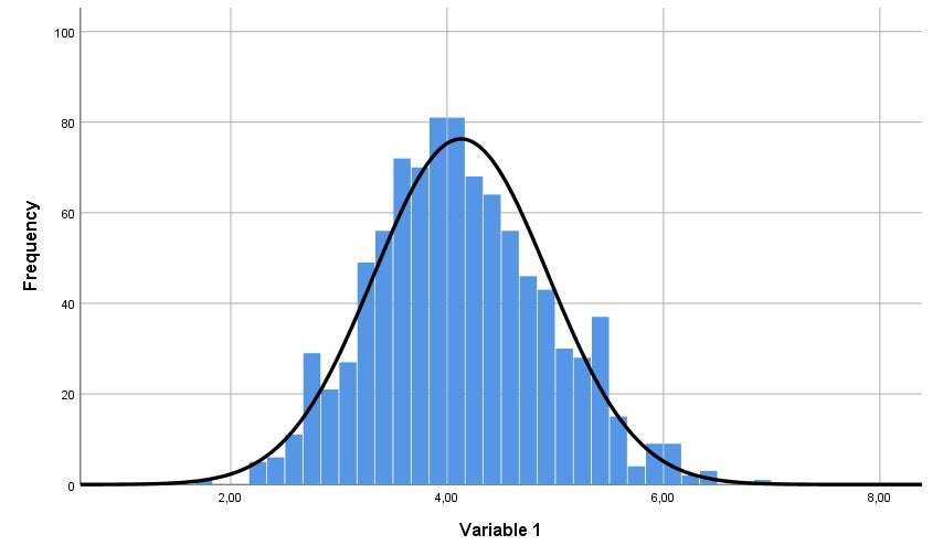
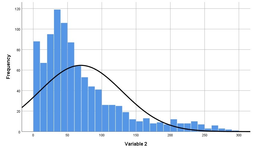
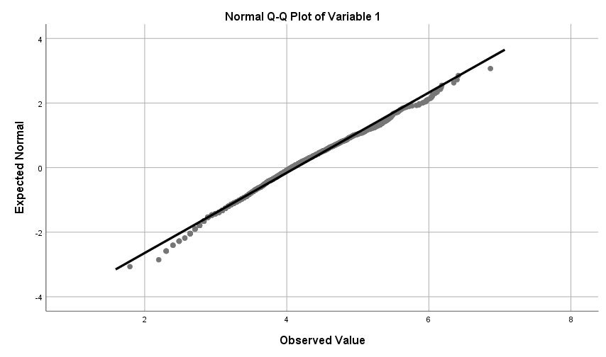
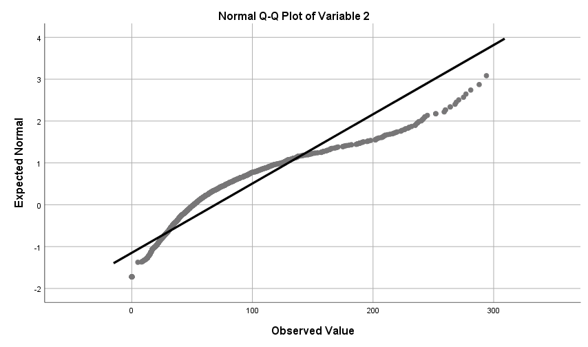
Categorizing (or 'grouping') data means we convert a quantitative variable into a categorical variable. This can be useful for instance when your quantitative outcome variable has severe problems with skewness, and you want to apply a statistical technique that assumes normality. We are going to take the variable delinquent behaviour as an example. This is a variable that is typically severely skewed to the right in samples; the majority of respondents generally report no (or very little) delinquent behaviour, whereas a few respondents will report a lot of delinquent behaviour. Since in this situation the assumption of normality of the data has been violated, recoding the variable into separate groups can be a solution to solve this problem. Other reasons for categorizing data are to help visualize an interaction between two quantitative predictors in multiple regression analysis, or when there is a clear theoretical ground for creating distinct groups of people based on a meaningful break point (e.g., grouping of 'depressed' versus 'not depressed' based on a cut-off score on a quantitative scale). 

Categorizing can be done in different ways. The most commonly used techniques are 1) the use of percentile scores, 2) median split, and 3) the use of pre-specified categories.

1. Percentile scores. One option to create groups is by using percentile scores. You could for instance ask SPSS to calculate quartiles, and thereby creating four different subgroups.

To create a new variable based on quartiles, go to:

• Transform > Rank Cases;
• Place the relevant variable(s) in the Variable (s) field;
• Click on Rank Types;
• Remove the check from 'Rank' and instead check Ntiles:4, and click on Continue;
• Click on 'Paste' and 'run' the syntax.
  

The new variable will appear on the rightmost column in the Data View, and on the bottom row in the Variable View. The new variable represents the four ranks; if a specific value on the original variable falls within the 25% lowest scores, then this case gets a value '1' here, all scores that fall between the 25% and 50% of the lowest scores receive the value '2', etc. The original variable is thus converted into a categorical (ordinal) variable.

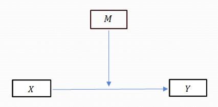
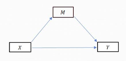
One of the uses of creating quartiles, is to make an interaction between two quantitative predictors visible. If this is your goal, then after you have converted one of the two quantitative predictors (or both) into quartiles, you can create a scatterplot in SPSS based on the new categorical variable.

To create the plot, go to:

• Graphs > Legacy Dialogs;
• Choose Simple Scatter and click 'Define';
• Place the quantitative predictor on the X-axis, the outcome variable on the Y-axis and the new categorical (quartile) variable in the box 'Set markers by', and then click on 'OK'. 
  

The graph will now be displayed in the output file.

• Double click on the figure, so the chart editor will open;
• Click on 'Elements' and 'Fit Line at Subgroups', and then close the chart editor.

(Note that there are also other ways to make an interaction between two quantitative predictors visible; either by using the Process module or through Modgraph. This latter option is a program to visualize/plot an interaction between two quantitative predictors. For this program you need to fill in relevant output values (like the mean and standard deviation of the predictors, and the regression coefficients), and then a graph will be drawn for you based on these values. You can access this program through: https://psychology.victoria.ac.nz/modgraph/modgraph.php)

2. Median split. With a median split you can convert a quantitative variable into a dichotomous variable (a categorical variable with only two possible values), based on the median of the variable in question. All values below the median then fall into one category, and all values above the median into another category. For an instruction on the median split technique in SPSS, go to: https://www.youtube.com/watch?v=B0nGVnQYy7k

3. Pre-specified categories. With pre-specified categories, you decide beforehand which scores will fall into a certain category (instead of letting the data decide the categories, like with median split or percentile scores). For instance, you can make different age groups (e.g., 10-19: adolescents, 20-64: adults, >64: seniors), based on logical pre-established distinctions. A challenge with this option is how to decide the specific ranges of each group, in the absence of a theoretical rationale. If there is no clear theoretical rationale, it is advised to use percentile scores or the median split option instead.

Categorization with pre-specified categories can be conducted in SPSS through the Compute command (Go to: 'Transform' --> 'Recode into different variables'). For a comprehensive instruction on how to categorize a variable, watch the following video: https://www.youtube.com/watch?v=nJ6nxRXRTHc

Note that categorizing variables can (and in most cases will) have consequences for the type of statistical technique you can use to test your hypothesis. Moreover, a disadvantage of categorizing variables, is that you 'lose' information, because you are grouping people or cases together, who might be very different from one another. By putting these cases together in one category, you cannot make a distinction between these cases anymore in your analysis. This typically results in a loss of power. Therefore, always make sure you have a legitimate reason to categorize a quantitative variable.

Which analysis technique is most suitable to test a given hypothesis, depends among other things on the number of independent and dependent variables in the hypothesis, the measurement level of the variables, and in case of categorical variables the number of categories. On this page you can find a diagram to help select the most suitable analysis technique for your study.

When you want to test a model with main effects AND an interaction effect, you often need to manually add the interaction term to your model. In other situations, you might want to remove an interaction-term from your model (for instance in a factorial ANOVA, when you are only interested in testing main effects).

How you can add or remove an interaction-term to your model in SPSS depends on the analysis technique that you are using. Below you'll find brief instructions on how this can be done for Multiple regression, Factorial ANOVA, and ANCOVA. 

Adding an interaction-term in Multiple regression
Note that when you want to test an interaction effect in Multiple regression with two quantitative predictors, it is best to center both quantitative predictors in order to prevent multicollinearity. See the section Centering for more information about this.

In order to test for an interaction effect between predictors in multiple regression you have to create a new interaction variable yourself and add this as a new variable to your data file. You can create the interaction term by taking the cross product of the two predictors:

• Choose Transform > Compute Variable;
• Give the Target Variable a logical name (e.g., Var1XVar2).
• Drag both independent variables into the Numeric Expression field with an asterisk in between. It now says: [Variable 1] * [Variable 2].
• Click on Paste and ‘run’ the syntax.

Now that you have created the interaction term, all you need to do is add it to you model, alongside your predictors. The interaction term is added to the model as an extra predictor/variable.

Adding an interaction-term in ANCOVA
When you perform an ANCOVA and you specifically want to test for an interaction between the factor and the covariate, you need to specify this while 'building' your model. Instruction on how to perform this in SPSS.

Adding or removing an interaction-term in Factorial ANOVA
When you perform an ANOVA in SPSS and you specifically want to test for an interaction between the factors, then all you need to do is enter the relevant factors in your model. SPSS will then automatically provide output for a model containing the main effects of the factors AND the interaction effect between the factors. If you, however, want to remove an interaction-term from your model (for instance when you are only interested in testing main effects, or when the interaction effect is not significant), then you need to specify this by 'building' your model. Instruction on how to perform this in SPSS.

What is the difference between moderation and mediation?
Moderation and Mediation are two different types of multivariate relationships. (Multivariate relationships are relationships with at least three variables.)

Moderation: The strength of a relationship between X and Y depends on the value of a third variable (the moderator).

Mediation: The relationship between X and Y proceeds via a third variable (the mediator).

Moderation. The strength of relationship between the independent variable (X) and the dependent variable (Y) depends on the value of a third variable (moderator). This type of relationship is also called an 'interaction'. In moderation, the moderator (M) affects the strength or the direction of the relationship between the variables X and Y. In other words, the relationship between X and Y looks different for different levels or values of the moderator. This is also described as 'an interaction between the variables X and M on the variable Y'. The moderator can be either a categorical or a quantitative variable. 

Schematic representation of moderation

Let's look at an example of moderation, with the variables STRESS (as the independent variable), GRADE (as the dependent variable) and GENDER (as the categorical moderator).

Is GENDER a moderator for the relationship between STRESS and GRADE? Let's assume we found that the relationship between STRESS and GRADE depends on GENDER. More specifically, for men there is a positive relationship between Stress and Grade; the higher the stress level in men, the higher their grade. For women the opposite relationship is found; a negative relationship: the higher the stress level in women, the lower their grade. In this case the relationship between STRESS and GRADE looks different for men compared to women. We then say that Gender moderates the relationship between Stress and Grade. In other words, there is an interaction between Gender and Stress in their effect on Grade.

Schematic representation of mediation

The relationship between the independent variable (X) and the dependent variable (Y) proceeds via a third variable (mediator). In mediation, the variable X affects the variable M, and this variable M in turn affects the variable Y. The variable M is called the mediator in this design, because it mediates the relationship between the variables X and Y. The mediator is also called 'the explaining factor in the relationship between X and Y'. 
 
Two types of mediation are typically distinguished:

• Partial Mediation. In Partial Mediation the relationship between the variables X and Y runs only partly via the mediator (this is called the 'indirect effect') and also partly directly between X and Y (this part is called the 'direct effect'). Partial mediation is also known as 'direct/indirect effect'. 
• Full Mediation. In Full Mediation the relationship between the variables X and Y proceeds completely via the mediator. In this case there is no direct effect present between X and Y. This is also called a 'chain reaction' and can be represented schematically as follows: 

Schematic representation of chain reaction

Let's look at an example of mediation, with the variables SOCIAL CONTACTS (as the independent variable), HAPPINESS (as the dependent variable) and SELF-ESTEEM (as the mediator).

Is SELF-ESTEEM a mediator for the relationship between SOCIAL CONTACTS and HAPPINESS? Let's assume we found that the relationship between SOCIAL CONTACTS and HAPPINESS proceeds via SELF-ESTEEM. More specifically, Social Contacts is positively related to Self-esteem; the more social contacts a person has, the higher that person's self-esteem. In turn, Self-esteem is positively related to Happiness; the higher a person's Self-esteem, the higher someone's happiness. In this case the relationship between SOCIAL CONTACTS and HAPPINESS proceeds via SELF-ESTEEM. We then say that Self-esteem mediates the relationship between Social contacts and Happiness.

Note that although in this example the proposed relationships all happened to be positive, relationships between variables in a mediation analysis could naturally also be negative instead of positive.
For more information about mediation, you could visit the website of David Kenny: http://davidakenny.net/cm/mediate.htm

How can I analyze a model with mediation or moderation in SPSS?
Moderation can be tested by conducting a Multiple regression analysis WITH an interaction effect. See the instructions on how to perform this in SPSS. Mediation can be tested by performing a series of simple and multiple regression analyses and reviewing the results step-by-step.

A more efficient way however to conduct Moderation and Mediation is via the modeling tool Process. This is a free downloadable plug-in for SPSS. The Process module offers a quicker and relatively easy way to analyze the data.

Go through the following steps to download and use the Process module in SPSS:

1. Download the process.spd file from the website and save the file on your computer. 
2. First make sure that SPSS is closed. Click on the start menu and select the folder 'IBM SPSS Statistics'. Look up the SPSS program and then click on it with the RIGHT mouse button. Click on 'Run as administrator' (with the left mouse button). It then asks if you allow the app to make changes to your device. Click 'yes'.
3. When SPSS has loaded, click on 'Extensions' >> Utilities >> Install Custom Dialog. (For older versions of SPSS, go to 'Utilities' >> Custom Dialogs >> Install Custom Dialog.) Select the process.spd file and click on 'open'. The module will now be installed in SPSS. 
4. If you now go to Analyze >> Regression, you should find the PROCESS module installed here.

In Process, Model 1 represents the Moderation analysis, and Model 4 represents the Mediation analysis.

Which assumptions should I always check?
Which assumptions are relevant to check depends on the analysis you're conducting. For an overview of some assumptions that are often relevant, go to (only in Dutch): https://wiki.uva.nl/methodologiewinkel/index.php/Hoofdpagina

What does Robustness of a test mean?
A test is said to be robust when it is largely unaffected by violations of assumptions, such as non-normal distribution shapes or unequal variances between groups.

What are nonparametric tests and when do you use them?
Nonparametric tests are tests that do not rely on the restrictive assumptions of parametric tests. Typically, nonparametric tests do not require interval/ratio level of measurement, normal distributions of scores, or equal variances between groups. Because many nonparametric procedures convert scores to ranks, outliers also have little impact on results. Nonparametric statistics can be used instead of parametric statistics, when assumptions for the parametric statistic have been violated. Some familiar examples of nonparametric statistics are Spearman's r, the Wilcoxon test, the sign test, and the Kruskall-Wallis test. The table on this page provides the most commonly used nonparametric substitutes for various parametric tests.

What are effect sizes?
Effect sizes are quantitative measures of the magnitude of an effect. It is an index of the strength of the relationship between two variables, or of the magnitude of the difference between means. The larger the effect size, the stronger the relationship between the variables.

Effect sizes help to determine whether a relationship between variables is meaningful or due to chance factors. An advantage of effect sizes over significance testing is that effect sizes are independent of sample size. Because sample size has a strong impact on the significance of a test, it is advised to consider the effect size in addition to the p-value/significance of a given test result. 

Examples of commonly used effect sizes are Pearson's r, (partial) r2, (partial) ɳ2 and Cohen's d.

How can I qualify effect sizes?
This table provides rules of thumb for the qualification of effect sizes.

What is bootstrapping and when do you use it?           
Bootstrapping is a statistical technique used to estimate the sampling distribution of parameters (such as the regression coefficient b). Bootstrapping does this by taking a new sample from the current sample many times, with replacement, and estimating the parameter per sample and looking at the distribution of parameters over these samples. Bootstrapping can for example be used in case of a fairly small sample, in case of non-normally distributed data in the sample, or in case of very complex models where the standard error of a parameter cannot be computed analytically. For a more comprehensive explanation about bootstrapping, you could read the following blog: https://statisticsbyjim.com/hypothesis-testing/bootstrapping/

What does statistical power entail and what is a power analysis?
Statistical power is the probability of obtaining a test statistic that is large enough to reject the null hypothesis, when the null hypothesis is actually false. Meaning, it is the probability of correctly rejecting the null hypothesis. In other words, it is the probability of finding a significant result in the sample when the effect also exists in the population. The higher the power of a given test, the better. There are three factors that affect the power: the (expected) effect size in the population, the sample size and the chosen significance level.

Power analysis is a procedure to help the researcher determine the smallest sample size that is suitable to detect the effect of a given test at the chosen level of significance. This is also called a priori power analysis. A priori power analysis is conducted prior to the research study, and is typically used in estimating what a sufficient sample size would be to achieve adequate power, given the estimated effect size in the population and the chosen significance level. A power analysis can be conducted with the programme G*Power, which can be downloaded from this website: http://www.gpower.hhu.de/

Power analysis is occasionally also conducted after the data are collected to determine the achieved power of a study given the sample size. This type of power analysis is called post-hoc power analysis or observed power analysis. Post-hoc power is interpreted as the retrospective power of an observed effect based on the sample size, observed effect size in the sample and the chosen significance level. Note however that using post hoc power to make a statement about the true power of your study is misleading; post-hoc power is basically just another way of representing the p-value of your study, and therefore does not provide any new information. For this reason, we do not recommend to calculate the post-hoc power. For a more elaborate discussion of the post-hoc power fallacy, you can read this blogpost.